The Poisson distribution

 

The Poisson distribution is a discrete probability distribution that expresses the probability of a given number of events occurring in a fixed interval of time and/or space if these events occur with a known average rate and independently of the time since the last event.

 

Example: let’s say that you are interested in knowing the probability that X cars  are going to pass in front your house in a given period of time.
To do that, you need to assume two things:

 

1)      Any period of time is no different than any other period of time;

2)      The number of cars that pass in one period doesn’t not affect the number of cars that will pass on the next period;

 

 

Give those assumptions, you need to find out how many cars on average pass in front of your house (that is your lambda  – λ).

If you want know the probability that K cars will pass, all you have to do is substitute λ and k on the formula bellow:

 

 

 

For example, lest say that the average is 9 cars and you want to know the probability that exactly 2 cars will pass:

λ =9

k=2

 

81 /2  * 0.000123   =  0.004998097

 

Or 0.5%

 

 

That same calculation can be can be achieved in R using the density dpois function:

 

dpois(2,9)

[1] 0.004998097

 

 

 

To compute cumulative probabilities (for example, probability of 0 or 1 or 2 or 3 cars ), we can use the ppois function (which is the same as summing all individual probabilities with dpois):

ppois(3,9)

[1] 0.02122649

 

sum(dpois(0:3,9))

[1]0.02122649

Probability of having seventeen or more cars passing by your house:

ppois(16, lambda=9, lower=FALSE) #upper tail 

[1] 0.01110591

OR

1-ppois(16, lambda=9) #lower tail

[1] 0.01110591

 

 

 

To finalise, we can simulate how many cars will pass on the next 10 hours:

rpois(10,9)

[1]  9  9 11 15  7  8  8 13 11  9

Understanding Association Rules

 

 

The goal of this post is to get a basic understanding on how the “association rules algorithms” work. Association rule learning is a popular and well researched method for discovering interesting relations between variables in large databases (wiki).

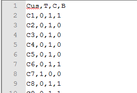
To do that, I’ll use a fictional dataset that consists of customers purchases on a coffee shop.  The data set is very simple and consists of 4 columns, the customer and whether he\she bought three different item on a particular purchase: tea, coffee, or bagel (represented by T, C and B respectively). Here’s an example (WordPress wont allow me to upload .csv files so I renamed it to .doc) where we can see that Customer C1 bought one coffee and one bagel; customers C2 to C5 bought only coffee and customer C6 bought coffee and bagel (the full data set contains 100 rows and can be downloaded from
here.

 

 

I’ll be using R to do some of the basic calculations so first I’ll load the dataset and do some counts (note that the data set indicates whether the item was bought or not, not the quantity, which doesn’t matter on this case – that’s why I’m using “count”):

 

df <- read.csv(“assoc_ex.csv”, header=TRUE) # Read the file with the data

dt <- data.table(df)#transform it into a data table

 

#Run some counts:

nrow(dt[T==1]) #Number of Customers that bought tea: 10

[1] 10

nrow(dt[C==1]) #Number of Customers that bought coffee: 91

[1] 91

nrow(dt[B==1]) #Number of Customers that bought bagel :51

[1] 51

 

 

To start we’ll calculate the {C} => {B} relationship, which can be read as “If Coffee is bought, the customer also buys Bagel”. To select interesting rules from the set of all possible rules, constraints on various measures of significance and interest can be used. The best-known constraints are minimum thresholds on support, confidence and Lift.

 

 

 

 

·         The support of an itemset X is defined as the proportion of transactions in the data set which contain the itemset. It is calculated by dividing the number of times the items C and B appear together by the number of observations.

o   Number of times Coffee and Bagel appear together (51 – 50 on their own and 1 with 3 all items) / 100 observations

o   S(C,B) -> N(C,B) / N  = 51/100 = 0.51

 

·         Confidence is calculated by dividing the number of times the items C and B appear together (51) by the number of times C appears on the dataset (91 – 40 alone, 50 with bagel and 1 with all 3 items). Confidence can be interpreted as an estimate of the conditional probability P(Y |X), the probability of finding the RHS of the rule in transactions under the condition that these transactions also contain the LHS.:

o   C(C,B) ->  N(C,B) / N(C) = 51/91 = 0.56

 

·         Lift is calculated by multiplying number of times the items C and B appear together (51) by the total number of observations (100) and dividing the result by the multiplication of the number of times C and B appear (51 and 91). Lift can be interpreted as the deviation of the support of the whole rule from the support expected under independence given the supports of the LHS and the RHS. Greater lift values indicate stronger associations.

o   L(C,B) ->  (N(C,B) * N) / (N(C) * N(B))   =  (51 * 100) / (91 * 51)  = 1.100

 

These rules can simply be implemented in R as:

nrow(dt[C==1 & B==1]) / nrow (dt) #Support

[1] 0.51

nrow(dt[C==1 & B==1]) / nrow(dt[C==1]) # Confidence

[1] 0.5604396

(nrow(dt[C==1 & B==1]) * nrow (dt)) / (nrow(dt[C==1]) * nrow(dt[B==1])) # Lift

[1] 1.098901

There are of course several rules we can calculate, for this example, I’ll calculated the following rules:

{C} => {B}
{C} => {T}
{B} => {C}
{C,B} => {T}

 

Which we already know the “counts” so I’ll load them into a few vectors and create a data-frame:

Vx  <- c("C","C","B", "CB")

Vy  <- c("B","T","C", "T")

Vnx <- c(91,91,51,51)

Vny <- c(51,10,91,10)

Vnxy <- c(51,1,51,1)

r <- data.frame(X = Vx, Y = Vy, Nx = Vnx, Ny = Vny, Nxy = Vnxy)  

 

Then calculate the values and do some formatting (N is hard coded here as 100):

r$Support <- r$Nxy/100

r$Confidence <- r$Nxy/ r$Nx

r$Lift <- (r$Nxy * 100) / (r$Nx * r$Ny)

r$Confidence  <-  format(round(r$Confidence , 2), nsmall = 2)   

r$Lift  <-  format(round(r$Lift , 2), nsmall = 2)   

r

   X Y Nx Ny Nxy Support Confidence Lift

1  C B 91 51  51    0.51       0.56 1.10

2  C T 91 10   1    0.01       0.01 0.11

3  B C 51 91  51    0.51       1.00 1.10

4 CB T 51 10   1    0.01       0.02 0.20

 

 

Association rules are usually required to satisfy a user-specified minimum support and a user-specified minimum confidence at the same time. If, let’s say, we want to impose a support of 0.1 and confidence of 0.8, we can come up with the rule that buying bagel is associated with buying coffee.

 

r<-data.table(r)

r[Support>=0.1 & Confidence >= 0.8]

   X Y Nx Ny Nxy Support Confidence Lift

1: B C 51 91  51    0.51       1.00 1.10

 

 

How to use R to run the same analysis:

We’ll be using R’s package “arules” to run the analysis. This package provides the infrastructure for representing, manipulating and analyzing transaction data and patterns (frequent itemsets and association rules). Also provides interfaces to C implementations of the association mining algorithms Apriori and Eclat by C. Borgelt.

 

install.packages("arules")

ibrary(arules) 

 

Initially I tried to use the package with the data on the format we’ve been working so far but I quickly noticed that having the items as flags is not the best way to use arules. The package has its own “transaction” class which represents transaction data used for mining itemsets or rules. It is a direct extension of class itemMatrix to store a binary incidence matrix, item labels, and optionally transaction IDs and user ID.

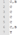
So here’s an example of what a transaction file looks like, where each row represents a transaction with its items separated by comas (or other separator).

 

By the way, the only reason why I have it on file is because I couldn’t find an easy way to transform data frames or tables to “transactions” – so I dumped the data into a file (on the desired format) and then used the read.transactions function to load the data into a “transaction” object. If anyone knows how to do this part without the dump\load I would be very interesting in learning.

 

So, this first part just add a column called products, which contains a letter for each product bought on the transaction.

products <- c()

for (i in 1:nrow(dt)) {

      t <- ifelse(dt[i,T==1],"T","")

      c <- ifelse(dt[i,C==1],",C","")

      b <- ifelse(dt[i,B==1],",B","")

      s <- paste(c(t,c,b), collapse = '')        

      s <- ifelse (substr(s,1,1)==",", substring(s, 2), substring(s, 1))    

      products[i] <- s  

}

dt<- cbind (dt, products)

head(dt)

   Cus T C B products

1:  C1 0 1 1      C,B

2:  C2 0 1 0        C

3:  C3 0 1 0        C

4:  C4 0 1 0        C

5:  C5 0 1 0        C

6:  C6 0 1 1      C,B

And here I do the write\read I mentioned (special attention to the row names, col names and quotes. If you don’t inform that, your data may be corrupt:

write.table(dt$products, file="dt.csv", row.names=FALSE, col.names=FALSE, sep=",", quote = FALSE)

t <- read.transactions("dt.csv",format="basket",sep=",")

inspect(t)

 

So here is how the object looks like:

    items

1   {B,  

     C}  

2   {C}  

3   {C}  

4   {C}  

5   {C}  

6   {B,  

     C}  

7   {T}  

 

And we can graphically see a frequency plot by running:

itemFrequencyPlot(t)

 

 

 

We’ll be using the apriori function to find the rules. The function mines frequent item sets, association rules or association hyper edges using the Apriori algorithm. Its default settings are:  minimum support: 0.1, minimum confidence: 0.8, maximum length of rules: 10 so if we run:

rules <- apriori(t)

quality(rules) <- round(quality(rules), digits=2) #rounding

inspect(rules)

We’ll quickly see the “who buys coffee also buys bagel” rule we manually calculated before:

inspect(rules)

  lhs    rhs support confidence lift

1 {}  => {C}    0.91       0.91  1.0

2 {B} => {C}    0.51       1.00  1.1

 

There are other interesting parameters that can be used like “parameter” where you can indicate minimum confidence, “control” where you can set the verbose of the algorithm an “appearance” which you can use to filter the rules (for example, if I remove the comment on the code bellow, I’d be filtering where the left hand side contains “C”):

 

rules <- apriori(t 

                  ,parameter = list(minlen=1, supp=0.1, conf=0.02)

                  #,appearance = list(lhs=c("C"))

                  ,control = list(verbose=F)

 )

rules <- sort(rules, by="confidence") #rules can also be sorted

install.packages("arulesViz")

library(arulesViz)

There are several different ways you can plot the rules. I’ll show some examples, but a cool way of looking at the rules is to use the interactive flag, which allows you to click on the rules and see its information

 

ibrary(arulesViz)

#plot(rules)

#plot(rules, method = "grouped")

#plot(rules, method = "graph")

#plot(rules, method = "graph", control = list(type = "items")) 

plot(rules, interactive=TRUE)

 

Interactive mode.

Select a region with two clicks!

Number of rules selected: 2 

  lhs    rhs support confidence     lift

1 {C} => {B}    0.51  0.5604396 1.098901

2 {}  => {B}    0.51  0.5100000 1.000000

 

 

Helpful Links:

http://en.wikibooks.org/wiki/Data_Mining_Algorithms_In_R/Frequent_Pattern_Mining/The_Apriori_Algorithm

http://en.wikipedia.org/wiki/Association_rule_learning

Using Matrix Multiplication to calculate the Intercept and the Slope

 

A different way to calculate the Intercept and slope of a function is to use Matrix Multiplication. Let’s try that with the dataset defined here. It’s a very simple dataset with one prediction (X) and one outcome (Y) where we know, from this post, that the Intercept is -1.336847 and the slope is 2.065414.

 

The first step is to derive 1 matrix and 1 vector from our data (which we will call X and Y). The matrix, X, will contain a column full of 1s and a column for each one of the predictions, in this example we only have 1, so it will be a 20 X 2 matrix (20 is the number of observations we have). The vector, Y, will contains only the outcomes, so it will be a 20 X 1 ”matrix”. Here is the R code to load them:

X = matrix(c(1,1,1,1,1,1,1,1,1,1,1,1,1,1,1,1,1,1,1,1,1,2,3,4,5,6,7,8,9,10,11,12,13,14,15,16,17,18,19,20), nrow=20, ncol=2)

Y = matrix(c(5,6,7,8,9,10,11,12,13,14,15,20,25,33,34,35,36,37,38,39), nrow=20, ncol=1)

X [,1] [,2] [1,]    1    1 [2,]    1    2 [3,]    1    3 [4,]    1    4 [5,]    1    5 [6,]    1    6 [7,]    1    7 [8,]    1    8 [9,]    1    9 [10,]    1   10 [11,]    1   11 [12,]    1   12 [13,]    1   13 [14,]    1   14 [15,]    1   15 [16,]    1   16 [17,]    1   17 [18,]    1   18 [19,]    1   19 [20,]    1   20

Y [,1] [1,]    5 [2,]    6 [3,]    7 [4,]    8 [5,]    9 [6,]   10 [7,]   11 [8,]   12 [9,]   13 [10,]   14 [11,]   15 [12,]   20 [13,]   25 [14,]   33 [15,]   34 [16,]   35 [17,]   36 [18,]   37 [19,]   38 [20,]   39

 

                Once we have those two objects, all we have to do is apply the formula bellow, which for the sake of simplicity, I did in 4 steps:

 

Multiply X by its transpose (the function “t” in R calculates the transpose of a matrix – Some matrix Algebra in R here):

A = t(X) %*% X

Calculate the inverse of A using the function “solve”:

B = solve(A)

 

Multiply the result by the transpose of X

C = B %*% t(X)

 

Multiply the result by the vector Y:

D = C %*% Y

 

The result will be a matrix containing the intercept and all the slopes:

D

          [,1]

[1,] -1.336842

[2,]  2.065414

 

 

 

On a slightly more complex example, let’s use the mtcars R dataset predict mpg using number of cylinders, horsepower and weight. First of all let’s run the regular lm function to see if we can match the values:

 

Library(mtcars)

lm(mpg ~ cyl + hp + wt, mtcars)

 

Call:

lm(formula = mpg ~ cyl + hp + wt, data = mtcars)

 

Coefficients:

(Intercept)          cyl           hp           wt 

   38.75179     -0.94162     -0.01804     -3.16697

 

So the function we are looking for is

y = 38.75179 -0.94162cyl – 0.01804hp -3.16697wt

 

#we are going to need the dplyr library to call the mutate function

library(dplyr)

#1)Create a copy of the mtcars dataset

aux = mtcars

#2)Extract just the columns we want:

aux = aux[,c("cyl","hp","wt")]

#3)Add a column with “one”

aux = mutate(aux, i=1)

#4)Convert into a matrix

X = data.matrix(aux[,c("i","cyl","hp","wt")])

5)Get our Y column from mtcars – which is the predicted values

Y = data.matrix(mtcars[,c("mpg")])

 

#6) At last, we can call the above formula in one go:

(solve(t(X) %*% X) %*% t(X)) %*% Y

          [,1]

i   38.7517874

cyl -0.9416168

hp  -0.0180381

wt  -3.1669731

 

And we can check that the values are the ones expected.

Tableau and R Interaction

 

This post’s goal is to show how to make tableau and R talk to each other.
In order to do that, you’ll need RServe running. To install it, you can open RStudio (or even just R), install the package from CRAM and then run the command RServe() to start the process:

 

install.packages("Rserve") library(Rserve)     Rserve() Starting Rserve…  "C:\…..\Rserve\libs\x64\Rserve.exe"

 

Once the server is running you can go to tableau and test the connection:

 

What we are going to do is look at the dbinom R function to calculate the probability of successes on X trials.

The Data Source that I’m using is the least important aspect of this demo, it just connects to an excel spreadsheet with rows numbered from 0 to 30. These are the number of successes we want to calculate the probability to

So when Number if successes = 1 the calculation result is the probability of getting 1 success on X number of trials.

For example, the probability of getting 1 success on 2 trials with 50% probability of success each trial is given by the formula:

> dbinom(x=1,size =2, prob = .5)

[1] 0.5

Which is 50%. If you toss 2 coins, you can get HH, HT, TH, TT, meaning that in 50% of the times you will get one success (heads being success for example)

Numbers of trials is defined by a parameter that goes from 0 to 30 so, clearly all values on “number of successes” bigger than “number of trials” will be zero after all the probability of getting 5 successes on 4 trials is 0.

The “Probability of Success” indicates how likely it is for ONE test to return positive. It’s set to 50% so we can imagine as if it was the toss of a coin for example. 

In order to calculate the result, we’ll create a table calculation and use the SCRIPT_REAL function (because the output is of type REAL) which itself has two parameters:

·         The first one is the R function with the and the parameters (x, size and prob) represented by .arg1, .arg2 and .arg3

·         The second is the tableau values that will be passes to the parameters

 

Here’s the calculation:

 

SCRIPT_REAL("

    dbinom(.arg1, size = .arg2, prob = .arg3)

",

    SUM([Number of Sucesses]),

    [Number of Trials],

    [Probability of Sucess]

)

We can see it working by dragging X (which I renamed to “number of successes” to rows and our calculation to values (of course, you have to create the two tableau parameters) and it will look like something like this (size 2, probability 50%) :

 

 

We can also create a distribution graph. To do that, create a copy of the sheet, right click on number if success, select “continuous” and change the graph type to “line” on the “Show Me” pane; Then, under “Marks” select “Bar”:

 

I also created a Boolean calculation called “DisplayonGraph” with the formula [Number of Sucesses]<=[Number of Trials] and used it as a filter set it to TRUE (in the graph sheet only) so your graph will reflect exactly the number of trials, otherwise it’d have a huge tail on the right if you inform few trials

Here is the end result:

 

I’d like to publish it to tableau public but unfortunately it doesn’t support R Scripts so click on the link bellow to download a version of the dashboard.

Download workbook (read details bellow)

FYI: I don’t know why but WordPress didn’t allow me to upload tableau files or even compressed files to the website so (please don’t judge me for this) I changed the file extension to .doc.

All you have to do is download the tableau_r.doc and rename it to .twbx (not twb – Its a package workbook)

The Binomial Distribution

 

In probability theory and statistics, the binomial distribution with parameters n and p is the discrete probability distribution of the number of successes in a sequence of n independent yes/no experiments, each of which yields success with probability p (source: wikipedia)

The dbinom function calculates the “probability of success” on a given experiment.

 

There are 3 main parameters, the number of successes for which you want to know the probability; the size (number of trials) and the probability of success on each trial.

 

So, for example, if we want to know the probability of success on the toss of a coin (let’s say “heads” mean success), we can do

dbinom(1, size = 1, prob = 1/2)

[1] 0.5

Clearly, the probability of “failure” (tails) is the same:

dbinom(0, size = 1, prob = 1/2)

[1] 0.5

 

 

If we want to know the probability of 2 heads on 2 tosses of a coin:

dbinom(2, size = 2, prob = 1/2)

[1] 0.25

 

The same way, one success can be calculated by

dbinom(1, size = 2, prob = 1/2)

0.5

Resulting 50%, which makes sense because when flipping a coin the possibilities are HH, HT, TH, TT and we can easily see that on 50% of the cases we have 1 success.

 

Second example, lets says you have a test to take with 5 multiple choice questions, each question has 5 alternatives.

What is the probability of getting exactly 3 questions right just answering them at random.

 

dbinom(3, size=5, prob=1/5)

[1] 0.0512

 

Its 5% so you better study!

 

 

It’s easier to verify this formula if we think as 1 hit in 2 questions with 3 alternatives each. So let’s say that the correct answer is C than B, we can guess:

AA
AB
AC
BA
BB
BC
CA
CB – we don’t want this because we want exactly 1 hit
CC

 

4 out of 9 = 4/9 = 0.44

dbinom(1, size=2, prob=1/3)

0.4444444

 

 

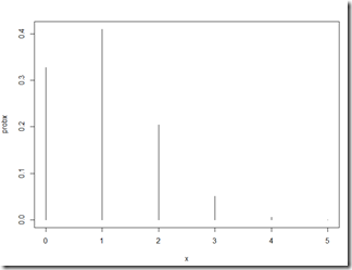
Back to the questions, we can see the probability of getting 0 to 5 questions right

 

x = seq(0,5,by=1)

probx = dbinom(x, size=5, prob = 1/5)

cbind(x, probx)

 

     x   probx

[1,] 0 0.32768

[2,] 1 0.40960

[3,] 2 0.20480

[4,] 3 0.05120

[5,] 4 0.00640

[6,] 5 0.00032

plot(x, probx, type = ‘h’)

Shiny

 

Shiny is a platform for creating interactive R programs embedded into a web page. I’ve been playing with it because it is part of the the “Developing Data Products” Coursera course.
This is a tutorial on how to create your first Shiny Application. It is a very simple one that will display n rows on the mtcars dataset.

Initially, it’s necessary to install the Shiny Package:

 

install.packages("shiny")

library(shiny)

A “shiny project” is simply a directory that needs to contain at least two files, the user interface (ui.R) where you specify how the application looks and the server (server.R) to controls what it does.

The project is run with the runApp() command. If we try to run it on an empty folder, we’ll get an error message:

> runApp()

Error in shinyAppDir(x): App dir must contain either app.R or server.R.

 

So what we need to do is to create both files on our working directory (or you can use any directory and its path as a parameter to the function). 

I’ve developed a very simple example that shows n rows of the mtcars dataset and summarizes its results.

 

This is how the ui.R file looks like:

 

shinyUI(

    pageWithSidebar(

        headerPanel("Hello Shiny – show me X rows on the mtcars dataset "),

       

        sidebarPanel(

            numericInput("amt", "Number of cars to view:", 5)

        ),

       

        mainPanel(

            verbatimTextOutput("summary"),

            tableOutput("myView")

        )

    )

And the server.R:

library(shiny)

library(datasets)

 

shinyServer(

                function(input, output) {

                                ds <- mtcars                      

 

                                output$myView <- renderTable({

                                                head(ds, n = input$amt)

                                })            

                               

                                output$summary <- renderPrint({                                          

                                                summary(head(ds, n = input$amt))

                                  })                          

                }

)

 

See that the variables amt, myView and summary are the communication variables between both “layers” (UI and Server). Calling runApp() will start the application:

> runApp()

Listening on http://127.0.0.1:5856

Distribution Shiny Apps:

 

A web App is not useful if you can’t distribute it. There are 2 main ways you can do that, using Shiny Server or a website like Shiny Apps.  Shiny Server runs on Linux only and I won’t be covering it here but all the information you need can be found on this link: http://www.rstudio.com/products/shiny/shiny-server/

If you want to deploy your app to the web, Shiny Apps (https://www.shinyapps.io) is a great option. Just go to the website, create an account and run the commands found here (https://www.shinyapps.io/admin/#/dashboard) on your R studio to install it.

 

 

Once you do it, all you have to do is call the deploy apss command and a browser will open with the application deployed:

 

> shinyapps::deployApp("c:\\git\\ShinyEx") Preparing to deploy application…DONE Uploading application bundle…DONE Deploying application: 28469… Waiting for task: 4160268   building: Building image: 109550   building: Installing packages   building: Installing files   building: Pushing image: 109550   deploying: Starting instances   rollforward: Activating new instances   success: Stopping old instances Application successfully deployed to http://dmenin.shinyapps.io/ShinyEx

 

This particular example can be found here: https://dmenin.shinyapps.io/ShinyEx/  

 

Basic Statistics in R

 

library(UsingR)

·         First let’s take a look at the data

·         We’ll be playing with the temperature variable so, to make things easier, let’s load it into a variable:

temp =airquality[,4]

 

·         Then let’s do a simple plot sorted by the temperature:

plot (sort(temp), xlab="Index", ylab = 'Temperature')

·         We can check the minimum, maximum, median and first and third quartile by creating a box plot:

boxplot(temp)

Or simply by running:

 

summary(temp)

   Min. 1st Qu.  Median    Mean 3rd Qu.    Max. 

  56.00   72.00   79.00   77.88   85.00   97.00 

 

 

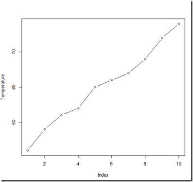
·         A functionality that I like a lot is adding a line connecting the points on the plot. Since we have a lot of points, I’ll be plotting the first 10 by doing temp[1:10] to better visualize the result. That can be achieved by using the “type = b” parameter

plot (sort(temp[1:10]), xlab="Index", ylab = 'Temperature', type = 'b')

·         The mean of the values can be calculated by the mean command. But let’s say we have an outlier on our dataset (this doesn’t make much sense on temperature, but it makes a lot of sense with salaries for example, where one person can earn a lot more than everyone else). A number that is so big, that we want to remove it because it is affecting mean calculation. To simulate that, I’ll sort the temp data and add an outlier with the “c” command:

temp2 <-sort(temp) #sort the data

temp2 <- c (temp2, 5000) # adds a new value to the integer vector

 

Then we can use the trim command which, in this case, removes 5% of the observations (from the top and the bottom)

mean(temp2)

[1] 109.8442

mean(temp2, trim=0.05)

[1] 78.19286

mean(temp)

[1] 77.88235

 

We can see that the second mean looks a lot closer to the actual mean than the first one.

 

·         Few other useful functions:

o   Range:

range (temp)

[1] 56 97

max(temp) - min(temp)

[1] 41

o   IQR (Interquartile range): difference between the third quartile and the first quartile

IQR(temp)

[1] 13

o   Variance 

var(temp)

[1] 89.59133

o   Standard Deviation:

sd(temp)

[1] 9.46527

sqrt(var(temp))

[1] 9.46527

round(sd(temp),1)

[1] 9.5

 

Basic R

 

Sharing a few notes, mainly commands, that helped me when I started playing with R:

Initial set up:

·         Download:

o   R: http://cran.r-project.org/bin/windows/base/

o   R Studio: http://www.rstudio.com/products/rstudio/download/

 

·         Display available packages to be installed:

a <- available.packages()

— Please select a CRAN mirror for use in this session —

 head(rownames(a),10)

 [1] "A3"          "ABCExtremes" "ABCoptim"    "ABCp2"       "ACCLMA"    

 [6] "ACD"         "ACNE"        "ACTCD"       "ADGofTest"   "ADM3" 

 

·         Installing a package – using the command line:
May need to extend the permissions on R’s folder ("C:/Program Files/R/R-3.1.1/library")

install.packages ("A3")

(Installs all dependencies as well)

Files temporary downloaded to:
C:\Users\<user>\AppData\Local\Temp\Rtmp6JVTkp\downloaded_packages

·         Installing a package – using R studio:

·         After installing a package you need to load it to be able to use the functions. The load is done using the library() command (you shouldn’t use quotes) – All dependencies are loaded as well:

 

 library(A3)

Loading required package: xtable

Loading required package: pbapply

 

·         Installing R tools and Dev tools
http://cran.r-project.org/bin/windows/Rtools/

install.packages("devtools")

library(devtools)

 

Basic Commands:

 

·         Check working directory:  getwd()

o   On the R console: Go to file -> Change dir to change the working directory

·         Read data: read.csv("test.csv")

·         Show what’s loaded on the workspace: ls()

·         Load a R function: source("mycode.r")

·         Show the object class:

o   x <- 0:6

o   class(x)

o   [1] "integer"

·         Create vector of objects:

o   c()

§  x <- c(0,2,0.4)

§  x

§  [1] 0.0 2.0 0.4

o   vector

§  x <- vector("numeric", length = 5)

§  x

§  [1] 0 0 0 0 0

·         Converting data

o   x <- 0:6

o    as.character(x)

o   [1] "0" "1" "2" "3" "4" "5" "6"

o   ——

o    x <- c("foo","foo2")

o    as.numeric(x)

o   [1] NA NA

o   Warning message:

o   NAs introduced by coercion

·         Matrices

o   Basic

§   m <- matrix(nrow = 2, ncol = 3)

§   m

     [,1] [,2] [,3]

[1,]   NA   NA   NA

[2,]   NA   NA   NA

§   dim(m)

[1] 2 3

§   attributes(m)

$dim

[1] 2 3

o   Option 2

§   m <- 1:10

§   m

 [1]  1  2  3  4  5  6  7  8  9 10

§   dim(m) <- c(2,5) #assign vector (2,5) to the dim attribute of m

§   m

     [,1] [,2] [,3] [,4] [,5]

[1,]    1    3    5    7    9

[2,]    2    4    6    8   10

o   Option 3 (binding)

§   x <- 1:3

§   y <- 10:12

§   foo1 <- cbind(x, y)

§   foo1

     x  y

[1,] 1 10

[2,] 2 11

[3,] 3 12

§   foo2 <- rbind (x,y)

§   foo2

  [,1] [,2] [,3]

x    1    2    3

y   10   11   12

·         Factors

o    x <- factor(c("one","two","two","three","one"))

o    x

[1] one   two   two   three one 

Levels: one three two

o    table(x)

x

  one three   two

    2     1     2  

o    unclass(x)

[1] 1 3 3 2 1

attr(,"levels")

[1] "one"   "three" "two" 

o   Setting the levels:

§   x <- factor(c("one","two","two","three","one"), levels = c("one", "two", "three"))

§   x

[1] one   two   two   three one 

Levels: one two three

·         Data Frames

o   x <- data.frame(foo = 1:4, bar = c(T,T,F,F))

o   x

  foo   bar

1   1  TRUE

2   2  TRUE

3   3 FALSE

4   4 FALSE

o    nrow(x)

[1] 4

o    ncol(x)

[1] 2

·         Names:

o   Objects

§   x <- 1:3

§   names(x)

NULL

§   names(x) <- c("foo","bar","norf")

§   x

 foo  bar norf

   1    2    3

o   Vector

§   x <- list(a=1,b=2,c=3)

§   x

$a

[1] 1

 

$b

[1] 2

 

$c

[1] 3

o   Matrices

§   m <- matrix (1:4, nrow =2, ncol=2)

§   dimnames(m) <- list(c("a","b"), c("c","d"))

§   m

  c d

a 1 3

b 2 4

·         Sub setting

o   a Matrix:

§   x <- matrix(1:6, 2, 3)

§   x[1, ]

[1] 1 3 5

§   x[1, , drop = FALSE]

§   [,1] [,2] [,3]

§  [1,] 1 3 5

o   A list:

§   x <- list (foo = 1:4, bar = 0.6)

§   x

$foo

[1] 1 2 3 4

 

$bar

[1] 0.6

 

§   x[1]     ##produces a list that contains 1,2,3,4

$foo

[1] 1 2 3 4

 

§   x[[1]]   ## produces just the sequence

[1] 1 2 3 4

o   List2

§   x <- list(foo = 1:4, bar = 0.6, baz = "hello")

§   x

$foo

[1] 1 2 3 4

 

$bar

[1] 0.6

 

$baz

[1] "hello"

 

§   name <- "foo" #variable with the string foo

§   x[[name]]

[1] 1 2 3 4

§   x[name]

$foo

[1] 1 2 3 4

o   Nested elements:

§   x <- list (a=list(1,2,3), b = list(4,5,6))

§   x[[c(1,3)]]

[1] 3

§   x[[c(2,1)]]

[1] 4

·         Partial Matching

o    x <- list(awrajhf = 1:5)

o    x

$awrajhf

[1] 1 2 3 4 5

o    x$a #matches the partial name

o   [1] 1 2 3 4 5

o    x[["a"]] #name doesn’t exist

NULL

o    x[["a", exact = FALSE]]

[1] 1 2 3 4 5

·         Removing NA values

o    x <- c(1,2,NA,4,NA,5)

o    bad <- is.na(x)

o    bad

[1] FALSE FALSE  TRUE FALSE  TRUE FALSE

o    y <- x[!bad]

 y

o   [1] 1 2 4 5

·         Removing NA values – 2 vectors

o    x <- c (1,2,NA,4,NA,5)

o    y <- c("a","b", NA,"d", NA, "f")

o    good <- complete.cases(x,y) #which positions are there that have both elements no missing

o    good

[1]  TRUE  TRUE FALSE  TRUE FALSE  TRUE

o    x[good]

[1] 1 2 4 5

o    y[good]

[1] "a" "b" "d" "f"

·         Read data

o   Pass the columns types:

§   initial <- read.table("foo.txt", nrows=10)

§   classes <-sapply(initial, class)

§   all <- read.table("foo.txt", colClasses = classes)

·         Dput-ting Objects:

o    y <- data.frame (a=1, b="a")

o    dput(y)#writes R code that can be used to reconstruct an R object

o    

o   structure(list(a = 1, b = structure(1L, .Label = "a", class = "factor")), .Names = c("a",

o   "b"), row.names = c(NA, -1L), class = "data.frame")

o    

o    dput(y, file="y.R")   # creates the y.R file

o    

o    new.z <- dget("y.R")

o    new.z

o     a b

o   1 1 a

o    

o    

o    foo <- dget("y.R")

o    foo

o     a b

·         Dumping Objects

o    x<-"foo"

o    y<-data.frame(a=1, b="a")

o    dump(c("x","y"),file ="data.R") # dump can be used on multple R objects

o    rm(x,y) # remove objects

 

o    x

Error: object ‘x’ not found

o    source("data.R")

o    x

[1] "foo"

·         Data Frame:

o   Print first n rows: head(mydf, n=2)

o   Last two rows: tail(mydf,2)

o   Number of rows: nrow(mydf)

o   Show line 47: mydf[47,]

o   Find number of missing values on colum:

§  length(which(is.na(mydf$Ozone)))

§   miss <- is.na(mydf[, "Ozone"])  ## A vector of TRUE/FALSE

§   sum(miss)

o   Subset of rows of the data frame where Ozone values are above 31 and Temp values are above 90:

§  mydf_sub <- subset(mydf, Ozone >31 & Temp >90)

o   Mean:

§  Option1:

·         mean(mydf[, "Ozone"], na.rm = TRUE)

§  Option2:

·         <- !is.na(mydf[, "Ozone"])

·          mean(mydf[use, "Ozone"])

 

 

·         CSV:

o    cameradata <- read.table ("c:\\rwd\\cameras\\cameras.csv", sep=",", header = TRUE)

o    head(cameradata)

·         Excel:

o    cameraData <- read.xlsx("cameras\\cameras.xlsx",sheetIndex=1,header=TRUE)

o    head(cameraData)

 

·          library(XML)

·         XML – basic

o    fileUrl <- http://www.w3schools.com/xml/simple.xml

o    doc <- xmlTreeParse(fileUrl,useInternal=TRUE)

o    rootNode <- xmlRoot(doc)

o    xmlName(rootNode)

o   [1] "breakfast_menu"

·         XML

o    xpathSApply(rootNode,"//name",xmlValue)

o   [1] "Belgian Waffles"             "Strawberry Belgian Waffles"  "Berry-Berry Belgian Waffles" "French Toast"                "Homestyle Breakfast"       

·         Json

o   install.packages("jsonlite")

o   library(jsonlite)

§  Dependency: install.packages(‘httr’)

o   jsonData <- fromJSON("https://api.github.com/users/jtleek/repos&quot;)

o    names(jsonData)   #shows the name of the attributes (names of the data frame)

§   names(jsonData$owner)

o   Writing data frames to JSON:

§  myjson <- toJSON(iris, pretty=TRUE)

§  cat(myjson)

o   Convert back to JSON

§  iris2 <- fromJSON(myjson)

§  head(iris2)

·         Data Table

o   data.table is an extension of data.frame. Should be used for fast aggregation of large data

§  http://cran.r-project.org/web/packages/data.table/index.html

o   install.packages("data.table")

o   library(data.table)

o   DF = data.frame(x=rnorm(9),y=rep(c("a","b","c"),each=3),z=rnorm(9))

o   DT = data.table(x=rnorm(9),y=rep(c("a","b","c"),each=3),z=rnorm(9))

o   Tables() #see all tables in memory

o    DT[2,] #Subsetting rows

o    DT[DT$y=="a",] # looking at rows based on criteria

o   DT[c(2,3)] #subsets second and third rows

o   Calculating values for variables with expressions

§  DT[,list(mean(x),sum(z))]  #applies mean and sum functions on variables x and z on the DT

o   Create table of the Y values:

§  DT[,table(y)]

o   Adding new columns: DT[,w:=z^2]

o   Set all values on Colum to 2: DT[, y:= 2]

o   Multiple operations

§  DT[,m:= {tmp <- (x+z); log2(tmp+5)}]    

§  It does both operations inside the brackets  and return the result

Regression Line and confidence interval

 

Here I expand a little the concept of regression line by adding statistic inference to the “foo” dataset that I defined here

Just to recap, we can do fit <- lm (Y ~ X, foo) to get the regression line’s coefficients and calculate the predicted point:

> fit$coef

(Intercept)           X 

  -1.336842    2.065414 

 

X	Y		Predicted Point
1	5		0.7286
2	6		2.794
3	7		4.8594
4	8		6.9248
5	9		8.9902
6	10		11.0556
7	11		13.121
8	12		15.1864
9	13		17.2518
10	14		19.3172
11	15		21.3826
12	20		23.448
13	25		25.5134
14	33		27.5788
15	34		29.6442
16	35		31.7096
17	36		33.775
18	37		35.8404
19	38		37.9058
20	39		39.9712

 

> summary(fit)

Call:

lm(formula = Y ~ X, data = foo)

Residuals:

    Min      1Q  Median      3Q     Max 

-6.3827 -2.3874  0.0519  2.4701  5.4211 

Coefficients:

            Estimate Std. Error t value Pr(>|t|)    

(Intercept)  -1.3368     1.6081  -0.831    0.417    

X             2.0654     0.1342  15.386 8.42e-12 ***

---

Signif. codes:  0 ‘***’ 0.001 ‘**’ 0.01 ‘*’ 0.05 ‘.’ 0.1 ‘ ’ 1

Residual standard error: 3.462 on 18 degrees of freedom

Multiple R-squared:  0.9293,   Adjusted R-squared:  0.9254 

F-statistic: 236.7 on 1 and 18 DF,  p-value: 8.42e-12

We can use the predict function to predict the values of x:

> X <- foo$X

> p<-predict(fit,data.frame(X), interval="confidence")

> p

 

 

Note that when we use interval=”confidence”, the lower and upper endpoints are displayed and that the “fit” column matches the values we calculated using the regression function.

 

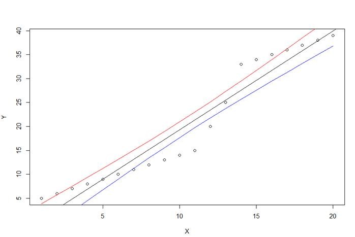
To finish, we can plot the data and the regression line:

> plot(foo$X, foo$Y, xlab="X", ylab="Y")

> abline(fit, foo)

 

And add 2 lines to represent the lower and upper confidence interval:

> lines(X,p[,2],col="blue") #Lower confidence interval

> lines(X,p[,3],col="red")  #upper confidence interval

 

T – Test for regression Coefficients

 

Getting the coefficients:

 

·         Prepare data:

library(UsingR);
data(diamond)

y <- diamond$price;
x <- diamond$carat;
n <- length(y)

 

·         Slope and intersect:

beta1 <- cor(y, x) * sd(y) / sd(x)

beta0 <- mean(y) – beta1 * mean(x)

·         Calculate the error:

e <- y – beta0 – beta1 * x #y – (beta1*x + beta0)

·         Calculate Sigma

> sigma <- sqrt(sum(e^2) / (n-2))

> sigma

[1] 31.84052

·         Calculate the sum of the squared Xs:
> ssx <- sum((x – mean(x))^2)
> ssx
[1] 0.1515667

·         Calculate the standard error for Beta0 and Beta1
> seBeta0 <- (1 / n + mean(x) ^ 2 / ssx) ^ .5 * sigma
> seBeta1 <- sigma / sqrt(ssx)
> seBeta0
[1] 17.31886
> seBeta1
[1] 81.78588

·         T distribution for hypothesis testing:
> tBeta0 <- beta0 / seBeta0;
> tBeta1 <- beta1 / seBeta1
> tBeta0
[1] -14.99094
> tBeta1
[1] 45.49715

·         P values (shouldn’t be bigger than 1):
> pBeta0 <- 2 * pt(abs(tBeta0), df = n – 2, lower.tail = FALSE)
> pBeta1 <- 2 * pt(abs(tBeta1), df = n – 2, lower.tail = FALSE)
> pBeta0
[1] 2.523271e-19
> pBeta1
[1] 6.75126e-40

 

 

Similarly:

> fit<-lm(y~x);

> summary(fit)$coefficients

 

 

Confidence Interval:

> sumCoef<-summary(fit)$coefficients

> sumCoef[2,1]+c(-1,1)*qt(.975,df=fit$df)*sumCoef[2,2]

[1] 3556.398 3885.651

 

With 95% confidence, we estimate that a 0.1 carat increase in diamond size results in a 355.6 to 388.6 increase in price in (Singapore) dollars.

In other words, the model predicts that a 0.16 carat diamond will cost 335.73, based on the confidence interval, we can assume with 95% confidence that a 0.26 (+0.1) diamond will cost between 691.33 (335.73 + 355.6) and 724.33 (335.73 + 388.6). This can be “verified” by looking at the predicted value for a 0.26 carat diamond, which is 707.83

 

Plotting the prediction Intervals:

Plot the points and the regression line:

> plot(x,y,frame=FALSE,xlab="Carat",ylab="Dollars",pch=21,col="black",bg="lightblue",cex=2)

> abline(fit,lwd=2)

 

Calculate X points and the predicted Y points:

> xVals<-seq(min(x),max(x),by=.01)

> yVals<-beta0+beta1*xVals

 

 

Calculate the standard error:

> se1<-sigma*sqrt(1/n+(xVals-mean(x))^2/ssx)

> se2<-sigma*sqrt(1+1/n+(xVals-mean(x))^2/ssx

 

> lines(xVals,yVals+2*se1)

> lines(xVals,yVals-2*se1)

> lines(xVals,yVals+2*se2)

> lines(xVals,yVals-2*se2)