The goal of this post is to get a basic understanding on how the “association rules algorithms” work. Association rule learning is a popular and well researched method for discovering interesting relations between variables in large databases (wiki).
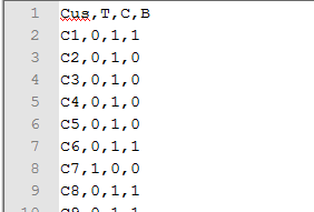
To do that, I’ll use a fictional dataset that consists of customers purchases on a coffee shop. The data set is very simple and consists of 4 columns, the customer and whether he\she bought three different item on a particular purchase: tea, coffee, or bagel (represented by T, C and B respectively). Here’s an example (WordPress wont allow me to upload .csv files so I renamed it to .doc) where we can see that Customer C1 bought one coffee and one bagel; customers C2 to C5 bought only coffee and customer C6 bought coffee and bagel (the full data set contains 100 rows and can be downloaded from
here.
I’ll be using R to do some of the basic calculations so first I’ll load the dataset and do some counts (note that the data set indicates whether the item was bought or not, not the quantity, which doesn’t matter on this case – that’s why I’m using “count”):
df <- read.csv(“assoc_ex.csv”, header=TRUE) # Read the file with the data
dt <- data.table(df)#transform it into a data table
#Run some counts:
nrow(dt[T==1]) #Number of Customers that bought tea: 10
[1] 10
nrow(dt[C==1]) #Number of Customers that bought coffee: 91
[1] 91
nrow(dt[B==1]) #Number of Customers that bought bagel :51
[1] 51
To start we’ll calculate the {C} => {B} relationship, which can be read as “If Coffee is bought, the customer also buys Bagel”. To select interesting rules from the set of all possible rules, constraints on various measures of significance and interest can be used. The best-known constraints are minimum thresholds on support, confidence and Lift.
· The support of an itemset X is defined as the proportion of transactions in the data set which contain the itemset. It is calculated by dividing the number of times the items C and B appear together by the number of observations.
o Number of times Coffee and Bagel appear together (51 – 50 on their own and 1 with 3 all items) / 100 observations
o S(C,B) -> N(C,B) / N = 51/100 = 0.51
· Confidence is calculated by dividing the number of times the items C and B appear together (51) by the number of times C appears on the dataset (91 – 40 alone, 50 with bagel and 1 with all 3 items). Confidence can be interpreted as an estimate of the conditional probability P(Y |X), the probability of finding the RHS of the rule in transactions under the condition that these transactions also contain the LHS.:
o C(C,B) -> N(C,B) / N(C) = 51/91 = 0.56
· Lift is calculated by multiplying number of times the items C and B appear together (51) by the total number of observations (100) and dividing the result by the multiplication of the number of times C and B appear (51 and 91). Lift can be interpreted as the deviation of the support of the whole rule from the support expected under independence given the supports of the LHS and the RHS. Greater lift values indicate stronger associations.
o L(C,B) -> (N(C,B) * N) / (N(C) * N(B)) = (51 * 100) / (91 * 51) = 1.100
These rules can simply be implemented in R as:
nrow(dt[C==1 & B==1]) / nrow (dt) #Support
[1] 0.51
nrow(dt[C==1 & B==1]) / nrow(dt[C==1]) # Confidence
[1] 0.5604396
(nrow(dt[C==1 & B==1]) * nrow (dt)) / (nrow(dt[C==1]) * nrow(dt[B==1])) # Lift
[1] 1.098901
There are of course several rules we can calculate, for this example, I’ll calculated the following rules:
{C} => {B}
{C} => {T}
{B} => {C}
{C,B} => {T}
Which we already know the “counts” so I’ll load them into a few vectors and create a data-frame:
Vx <- c("C","C","B", "CB")
Vy <- c("B","T","C", "T")
Vnx <- c(91,91,51,51)
Vny <- c(51,10,91,10)
Vnxy <- c(51,1,51,1)
r <- data.frame(X = Vx, Y = Vy, Nx = Vnx, Ny = Vny, Nxy = Vnxy)
Then calculate the values and do some formatting (N is hard coded here as 100):
r$Support <- r$Nxy/100
r$Confidence <- r$Nxy/ r$Nx
r$Lift <- (r$Nxy * 100) / (r$Nx * r$Ny)
r$Confidence <- format(round(r$Confidence , 2), nsmall = 2)
r$Lift <- format(round(r$Lift , 2), nsmall = 2)
r
X Y Nx Ny Nxy Support Confidence Lift
1 C B 91 51 51 0.51 0.56 1.10
2 C T 91 10 1 0.01 0.01 0.11
3 B C 51 91 51 0.51 1.00 1.10
4 CB T 51 10 1 0.01 0.02 0.20
Association rules are usually required to satisfy a user-specified minimum support and a user-specified minimum confidence at the same time. If, let’s say, we want to impose a support of 0.1 and confidence of 0.8, we can come up with the rule that buying bagel is associated with buying coffee.
r<-data.table(r)
r[Support>=0.1 & Confidence >= 0.8]
X Y Nx Ny Nxy Support Confidence Lift
1: B C 51 91 51 0.51 1.00 1.10
How to use R to run the same analysis:
We’ll be using R’s package “arules” to run the analysis. This package provides the infrastructure for representing, manipulating and analyzing transaction data and patterns (frequent itemsets and association rules). Also provides interfaces to C implementations of the association mining algorithms Apriori and Eclat by C. Borgelt.
install.packages("arules")
ibrary(arules)
Initially I tried to use the package with the data on the format we’ve been working so far but I quickly noticed that having the items as flags is not the best way to use arules. The package has its own “transaction” class which represents transaction data used for mining itemsets or rules. It is a direct extension of class itemMatrix to store a binary incidence matrix, item labels, and optionally transaction IDs and user ID.
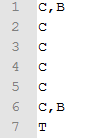
So here’s an example of what a transaction file looks like, where each row represents a transaction with its items separated by comas (or other separator).
By the way, the only reason why I have it on file is because I couldn’t find an easy way to transform data frames or tables to “transactions” – so I dumped the data into a file (on the desired format) and then used the read.transactions function to load the data into a “transaction” object. If anyone knows how to do this part without the dump\load I would be very interesting in learning.
So, this first part just add a column called products, which contains a letter for each product bought on the transaction.
products <- c()
for (i in 1:nrow(dt)) {
t <- ifelse(dt[i,T==1],"T","")
c <- ifelse(dt[i,C==1],",C","")
b <- ifelse(dt[i,B==1],",B","")
s <- paste(c(t,c,b), collapse = '')
s <- ifelse (substr(s,1,1)==",", substring(s, 2), substring(s, 1))
products[i] <- s
}
dt<- cbind (dt, products)
head(dt)
Cus T C B products
1: C1 0 1 1 C,B
2: C2 0 1 0 C
3: C3 0 1 0 C
4: C4 0 1 0 C
5: C5 0 1 0 C
6: C6 0 1 1 C,B
And here I do the write\read I mentioned (special attention to the row names, col names and quotes. If you don’t inform that, your data may be corrupt:
write.table(dt$products, file="dt.csv", row.names=FALSE, col.names=FALSE, sep=",", quote = FALSE)
t <- read.transactions("dt.csv",format="basket",sep=",")
inspect(t)
So here is how the object looks like:
items
1 {B,
C}
2 {C}
3 {C}
4 {C}
5 {C}
6 {B,
C}
7 {T}
And we can graphically see a frequency plot by running:
itemFrequencyPlot(t)
We’ll be using the apriori function to find the rules. The function mines frequent item sets, association rules or association hyper edges using the Apriori algorithm. Its default settings are: minimum support: 0.1, minimum confidence: 0.8, maximum length of rules: 10 so if we run:
rules <- apriori(t)

quality(rules) <- round(quality(rules), digits=2) #rounding
inspect(rules)
We’ll quickly see the “who buys coffee also buys bagel” rule we manually calculated before:
inspect(rules)
lhs rhs support confidence lift
1 {} => {C} 0.91 0.91 1.0
2 {B} => {C} 0.51 1.00 1.1
There are other interesting parameters that can be used like “parameter” where you can indicate minimum confidence, “control” where you can set the verbose of the algorithm an “appearance” which you can use to filter the rules (for example, if I remove the comment on the code bellow, I’d be filtering where the left hand side contains “C”):
rules <- apriori(t
,parameter = list(minlen=1, supp=0.1, conf=0.02)
#,appearance = list(lhs=c("C"))
,control = list(verbose=F)
 )

rules <- sort(rules, by="confidence") #rules can also be sorted
install.packages("arulesViz")
library(arulesViz)
There are several different ways you can plot the rules. I’ll show some examples, but a cool way of looking at the rules is to use the interactive flag, which allows you to click on the rules and see its information
ibrary(arulesViz)
#plot(rules)
#plot(rules, method = "grouped")
#plot(rules, method = "graph")
#plot(rules, method = "graph", control = list(type = "items"))
plot(rules, interactive=TRUE)
Interactive mode.
Select a region with two clicks!
Number of rules selected: 2
lhs rhs support confidence lift
1 {C} => {B} 0.51 0.5604396 1.098901
2 {} => {B} 0.51 0.5100000 1.000000
Helpful Links:
http://en.wikibooks.org/wiki/Data_Mining_Algorithms_In_R/Frequent_Pattern_Mining/The_Apriori_Algorithm


